
From Performance Curve to Trusted Model


To simulate a full data center, you need trustworthy component models. Vendors give you performance curves. Here’s how to turn one into the other.
Hyperscalers, commissioning engineers, and cooling vendors are all trying to build the same thing: a system model of a full data center that behaves like the real one. A digital twin, if you want the term. It needs to be accurate enough to trust for decisions and fast enough to actually run.
Part of what’s driving this is that the load is no longer steady. AI workloads are bursty by nature. A job can saturate a rack in seconds, then drop, then spike again. Power demand at the rack level is no longer a steady number you can design around once. The cooling system doesn’t respond to those swings all at once. The chip reacts in milliseconds, the coolant loop in seconds to minutes, and the facility plant over minutes to hours. If you want to know whether your cooling system holds through a transient, you have to see all three together, which means a model of the whole system running fast enough to simulate the event.
That is a high bar for the components inside it. Each has to be accurate across its operating range and efficient enough to run thousands of times. The cleanest path would be a physics model of every unit built from vendor design details. But those details usually are not available, vendors rarely share enough information to build such a model, and nobody has time to reverse-engineer it. So you work with what you do have: the performance curve on the product sheet. This is what the coolant distribution unit (CDU) calibration workflow in Modelon’s Data Center Library (DCL) is built for: turning that curve into a component model you can trust inside the larger system.
What You’re Actually Working With
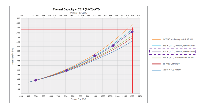
Here’s a typical scenario. You’re evaluating a CDU for a high-density rack deployment. The vendor datasheet gives you a family of curves, with heat rejection on the Y-axis, FWS flow rate on the X-axis, and one curve per ASHRAE W-class supply temperature.
What the datasheet doesn’t tell you is how thermal resistance splits between the TCS side and the FWS side, how quickly heat transfer degrades as flow drops below nominal, how viscosity changes at different water temperatures affect heat exchanger behavior, or what the pressure drop actually looks like across the operating range.
A generic model makes assumptions about all of this. Sometimes those assumptions are close enough. Often they are not, and you may not discover the discrepancy until you are comparing results against commissioning data. That is not the ideal time to find out. Here’s what makes calibration work. That performance curve is more than a specification to check against. It is the integrated result of all the physics the vendor didn’t write down: the resistances, heat exchanger falloff, fluid behavior, and everything else measured and rolled into one line. You cannot read those individual values directly from the plot. But you can fit a physics-based model to it. Once the model reproduces the curve, its internal parameters stop being guesses. Calibration doesn’t add data you do not have. It extracts information that is already embedded in the data you do have.
What’s Being Calibrated
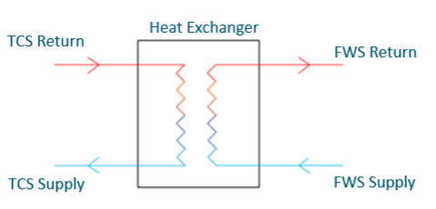
The CDU model in DCL uses a two-resistance UA-NTU formulation, where heat transfer is governed by:
1/UA = R_TCS + R_FWS
Each resistance varies with mass flow and fluid temperature. The parameters that calibration fits are:
- UA_corr: A global multiplier that corrects any uniform offset between model and reality.
- r_TCS: The fraction of total thermal resistance that sits on the TCS side.
- n_mu_TCS / n_mu_FWS: Viscosity exponents controlling how heat transfer responds to temperature changes on each loop.
- CF_Friction: Pressure-drop correction factors, one for each side.
The goal is to find the combination that makes the model match the vendor curve across the operating envelope, not just at nominal conditions.
The Workflow

1. Digitize the Datasheet
Start with the vendor’s performance plot. Use a digitization tool such as WebPlotDigitizer to extract (x, y) data pairs, then organize them into an Excel file using SI units: kg/s, W, and K. The column structure needs to match what the Modelon Calibration Library expects, so creating a template once can save time later.
2. Identify Your Datasheet Type
This matters more than it appears. A datasheet with multiple supply temperatures contains information about how the heat exchanger responds to viscosity changes, while one with a single supply temperature does not. That determines which parameters are identifiable. If the FWS supply temperature never varies, there is no signal to fit the FWS viscosity exponent, so it remains at its default value. Knowing that up front prevents you from chasing a parameter that the data cannot constrain.
3. Configure the Test Bench
DCL includes a CalibrationTestBench model for each supported CDU. It replicates the boundary conditions implied by the vendor’s test setup, including PID-controlled TCS supply temperature and specified FWS supply conditions. This is the model that the Calibration Library optimizes against.
4. Set Up Reference Files
Use the Reference File Loader in Modelon Impact to map your Excel columns to model variable paths. This creates the structured reference dataset against which the calibration minimizes error.
5. Run the Calibration
The Modelon Calibration Library handles the optimization. You specify which parameters to vary, set their bounds, and choose which outputs to fit, typically heat rejection and pressure drop if the datasheet includes it. The tool runs iteratively and returns the parameter set that best matches the reference data.
6. Verify
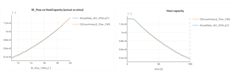
The VerificationTestBench sweeps across the full operating range and compares simulation results against vendor reference data at each point. This is where you see how the calibration actually performed.
Three CDUs, One Different Outcome
Real results are worth examining because they reveal as much about the limitations as the successes. The numbers below compare the calibrated model against the vendor’s own reference data. They represent the remaining error after fitting, not before.
Vertiv Liebert XDU1350 (~1.3 MW)
The Vertiv datasheet covers all four ASHRAE W-classes with multiple flow points per temperature. That provides enough information to fit both viscosity exponents in a single combined run, resulting in one parameter set valid across W1 through W4.
The result is 2% to 5% error in the normal operating range. At very low FWS flow rates, the model diverges more, reaching around 20%. This reflects a structural limit in the power-law flow relationship rather than a calibration failure. Those very low flows typically appear in redundancy or turndown scenarios rather than normal operation. That is worth keeping in mind if those scenarios are important to your analysis, since that is where the model has the greatest uncertainty.
OCP 2 MW CDU (Deschutes): Best Case
The Deschutes is a symmetric design with balanced thermal resistance and no internal pump. Its datasheet covers W1 through W4 with good flow resolution. This calibration achieved less than 1.4% error in heat rejection across the full flow range.
When you have multi-temperature data combined with solid flow coverage, calibration can come very close to reproducing vendor measurements.
nVent CDU800 (~800 kW): Where Data Limits You
The CDU800 provides a useful counterexample. Its datasheet contains only three discrete flow combinations, and the UA-flow relationship for this unit is steep, with roughly a 40% drop in UA for a 22% reduction in flow. Three operating points are not enough to fully characterize that behavior.
For W2, the only temperature the datasheet actually covers, errors range from 3% to 8%. W1 and W3 records were derived by shifting the W2 data to different supply temperatures because the vendor only published one chart. That approximation introduces its own uncertainty, and errors reach 26% at the extremes.
The calibration did not introduce that error. It was already present in the available data before the optimizer ran. If you are using this unit in a system model, keep studies close to nominal conditions and treat boundary-condition predictions with appropriate caution. A fourth unit, the Refroid SentraFlo, falls between these cases at roughly 1% to 5% error. Across all four examples, the pattern is consistent: the accuracy you get out is determined by the quality and coverage of the data the vendor put in.
What Changes with a Calibrated Model
A calibrated model behaves in a way that can be traced back to what the vendor actually measured across the operating range. It is not anchored to a single nominal point and assumed valid everywhere else. That affects the decisions you make with it. FWS supply temperature requirements become grounded in real heat exchanger performance. Pump sizing can be based on pressure-drop behavior that reflects the actual unit. Cooling margins become easier to defend in a design review, provided you stay within the range covered by the datasheet. The nVent example serves as a reminder: a calibrated model is trustworthy where the data supports it and transparent about where it does not.
Because the calibrated CDU lives within the library, it can be inserted directly into a full system model. That brings the discussion back to where we started. The component you fit to a vendor curve becomes one accurate, fast-running part of the system twin. When you simulate a transient, such as an AI load swing propagating through the chip, loop, and plant, the CDU’s contribution is grounded in measured performance rather than default assumptions. Calibration is not a side exercise. It is the front end of every system-level metric you care about, including capacity headroom, W-class tradeoffs, and overall system resilience during load fluctuations.
The Method Isn’t Really About CDUs
There is nothing about this approach that is specific to coolant distribution units. A chiller datasheet or a CRAH performance table presents the same challenge: a measured curve standing in for physics that the vendor never published, paired with a physics-based model whose parameters can be fitted rather than guessed. The same logic applies directly.
Today, DCL provides this workflow for CDUs, complete with test benches and calibrated records. The broader pattern applies to any component with a published performance curve. The method stays the same. Only the test bench setup changes.
Supported Equipment in the Data Center Library
| CDU | Capacity | Error (Nominal Range) |
|---|---|---|
| Vertiv Liebert XDU1350 | 1~1.3 MW | 2-5% |
| OCP 2 MW CDU (Deschutes) | 2 MW | <1.4% |
| nVent CDU800 | ~800 kW | 3-8% near nominal |
| Refroid SentraFlo ATD4 | 121.2-2.1 MW | ~1-5% |
Each ships with its calibration test bench, verification model, and calibrated parameter records. If you have a different CDU and a datasheet, the workflow remains the same. Configuring the test bench is the part that requires effort; the calibration itself is automated.
Component names reference real products for identification purposes only. Modelon is not affiliated with or endorsed by the respective manufacturers. All performance data is drawn from publicly available vendor datasheets.
References
Vendor datasheets
• Vertiv. Liebert XDU1350 Coolant Distribution Unit — Product Datasheet. Vertiv Group Corp.
• nVent. CDU800 Liquid-to-Liquid Coolant Distribution Unit — Specification Sheet.
• Open Compute Project. Project Deschutes — 2 MW Coolant Distribution Unit Specification, 2025.
• Refroid. SentraFlo ATD4 — In-Row Liquid-to-Liquid Coolant Distribution Unit Datasheet.
Standards
• ASHRAE Technical Committee 9.9. Liquid Cooling Guidelines for Datacom Equipment Centers. American Society of Heating, Refrigerating and Air-Conditioning Engineers. (Defines W1–W4 facility water supply temperature classes: 17 °C, 27 °C, 32 °C, 45 °C)