Co-simulation using the open-source Python package PyFMI
Different simulation and modeling tools often use their own definition of how a model is represented and how model data is stored. Complications arise when trying to model parts in one tool and importing the resulting model in another tool, or when trying to verify a result by using a different simulation tool.
The Functional Mock-up Interface (FMI) is a standard to provide a unified model execution interface for exchanging dynamic system models between modeling tools and simulation tools. The standard has been a great success as numerous tools, both open source and commercial, have adopted it, as well as having gained widespread adoption among users.
With the FMI standard, simulation of coupled dynamical systems in a co-simulation setting is made possible. In this blog I introduce PyFMI and its capabilities related to simulation of coupled systems.
This new tool has been the focus of my recently completed PhD work – a collaboration between Modelon and Lund University.
Stable simulations of coupled dynamic systems constructed using models from different FMI-compatible tools
What is PyFMI and what is it good for?
PyFMI is an open source Python package offered by Modelon aimed at working with models compliant with the FMI standard. It is designed to provide a high-level, easy to use, interface for working with FMUs.
The package is not only a mapping of the FMI interface to Python, it provides much of the functionality needed to perform various experiments for both evaluating the complex dynamical system model by itself, but also for evaluating the physics that the model represents. The experiments include linearization, simulation and parameter estimation.
PyFMI supports both FMI 1.0 and FMI 2.0 and the two different model types, model exchange and co-simulation. Furthermore, PyFMI includes a master algorithm for simulation of coupled FMUs following the co-simulation standard using FMI 2.0. In this article, the focus is on the included master algorithm.
The master algorithm
The FMI standard does not specify a co-simulation master, i.e. the algorithm responsible for controlling the overall simulation of the coupled system.
The classical algorithm for performing a co-simulation is to let each separate model perform a simulation step, exchange information between the models and then take another step.
The success of this algorithm is dependent on how the models are defined. In order to perform a stable and efficient simulation both the models and the algorithm need to be taken into account.
In PyFMI, a master algorithm has been implemented that includes the latest research related to co-simulation and one of the advances includes stabilization of simulations where the classical algorithm fails.
Example: Simulation of coupled inertias
This example demonstrates the use of the master algorithm on a coupled system available in the Modelica Standard Library (MSL).
The example was selected in order to demonstrate the use of PyFMI’s master algorithm on a small test system. The model that we focus on is GenerationOfFMUs from the examples in the rotational section, see Figure 1. The model contains two rotational bodies connected with a shaft – a pattern you often see in automotive and power industries.
Even though the coupled system in the example seems trivial, it is very useful for pointing to the difficulties one can encounter when performing co-simulation and – what concerns PyFMI – the need for using a sophisticated and still handy to use algorithm.
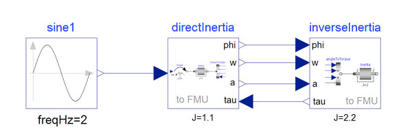
Figure 1: Coupled rotational bodies from the example GenerationOfFMUs from the MSL
Difficulty with classical co-simulations
The model is problematic in a co-simulation setting, as there is direct feed-through in both the component directInertia and the inverseInertia, i.e. the input directly impacts the output.
This feed-through may result in a severe degradation of the simulation or even simulation failure when using the classical co-simulation approach.
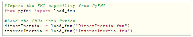
In the following script, it is assumed that co-simulation FMUs of both the directInertia and the inverseInertia are available and that they follow FMI 2.0.
Workflow with PyFMI
In order to work with the FMUs from Python, we first need to import the capability from the PyFMI package and then invoke the method load_fmu to load the FMUs into Python.
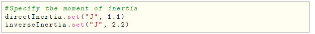
Furthermore, we set the moment of inertia in both models to be equivalent to the values in the MSL example.
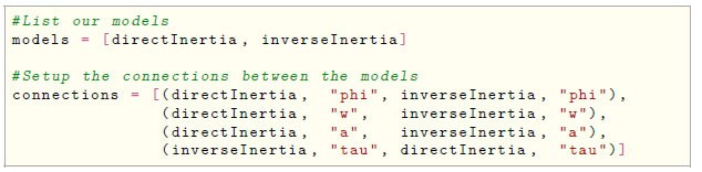
Now that the models are loaded and values set, we focus on constructing the coupled system. The model directInertia has three outputs, angle, angular velocity and angular acceleration while the inverseInertia has one output, torque.
These couplings are specified in a list which we later on will use as inputs to the master algorithm. The different models involved in the coupled system are also listed.
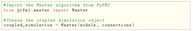
Using the connections and the list of the models we can now create our simulation object for the coupled system.
The master algorithm is controlled using options available on the simulation object. A dictionary with the available options is easily retrieved and options are easily set as shown below.
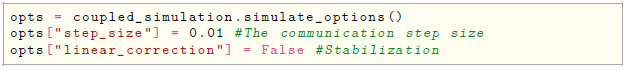
Information about the different options are available on the opts object.

In Figure 1 it was shown that the model is driven by an input signal. This signal also needs to be specified as an input to our coupled system.
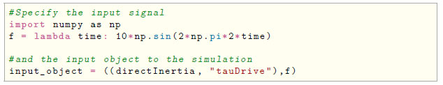
Now that the simulation object has been created, simulation options specified and input object defined we can invoke the simulation method to simulate the system.

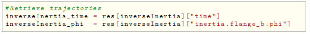
The returned resulting trajectories can easily be retrieved from the res object.
Stable systems simulations with PyFMI – the main benefit
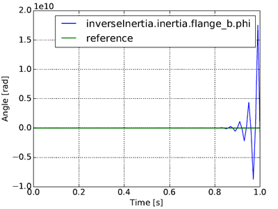
Simulating this coupled system using the classical approach results in an unstable simulation as is shown in Figure 2. The trajectories explodes due to the direct feed-through in the models.
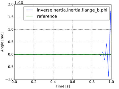
Figure 2: Simulation of the coupled inertias highlighted in the MSL example GenerationOfFMUs using the classical algorithm. As shown, the trajectories explode and the simulation is unstable
With FMI 2.0, the ability to use directional derivatives of the outputs with respect to inputs is available. Using these derivatives, the master algorithm can stabilize the simulation — see Figure 3.
In this figure results are shown when the directional derivatives have been used to stabilize the simulation (i.e the option linear correction has been set to True). The effectiveness of the method for stabilization is reflected in the agreement between the reference case and the simulation.
Note that the directional derivatives is an optional feature in the FMI standard and not all exporting tools support the feature.
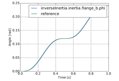
Figure 3: Simulation of the coupled inertias highlighted in the MSL example GenerationOfFMUs. The simulation leverages the directional derivatives to stabilize the simulation and as shown, give a good agreement with the reference result.
Try out PyFMI!
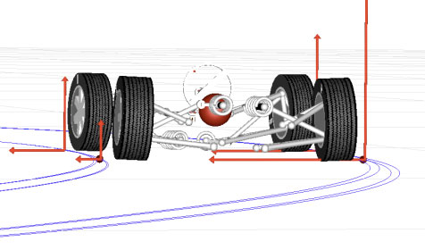
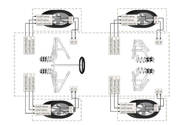
Co-simulation in regards to FMI is increasingly being used to connect models from different tools in order to understand the full system behavior, be it in simulation of smart grids or simulation of vehicles systems. Find here a co-simulation overview.
PyFMI is the Python package for working with FMUs. The package includes the latest research related to simulation of coupled systems.
If you have models in different tools that support FMI and the interest is in the system behavior, try out PyFMI!
PyFMI is an open source package (LGPL license) developed by Modelon.
For further details don’t hesitate to contact us!